Unravelling the Depths of Data Warehouses

In this article, we see the inner workings of data warehousing, unraveling the algorithms behind analytical processing.

The convergence of technology and analytics unlocks the hidden potential within vast datasets. In this article, we see the inner workings of data warehousing, unraveling the algorithms behind analytical processing. As a young professional with a background in data engineering, I am excited to guide you through key topics that form the backbone of analytical insights.

Star and Snowflake Schema for Analytics:

The star schema and snowflake schema are data warehouse design patterns that help simplify analytics and reporting.

Star Schema

• It has one large central fact table that contains business measurements and metrics (like sales amounts).

• Surrounding the fact table are smaller dimension tables that contain reference information (like date, product, customer details).

• The primary keys from each dimension table are referred to as foreign keys in the fact table. This allows them to be joined.

Consider a scenario where we are analyzing data related to car sales:

In this star schema:

• The Sales fact table holds quantitative data like sales_amount and quantity_sold.

• The Date Dimension provides information about the date of the sale, allowing for time-based analysis.

• The Car Model Dimension contains details about the car model, facilitating analysis based on different car attributes.

• The Customer Dimension stores information about the customer, enabling customer-centric analysis.

The fact table is connected to each dimension table through foreign key relationships, forming a star-like structure. This design simplifies querying and analysis, as each dimension is directly connected to the central fact table, making it easy to retrieve information for reporting and decision-making purposes.

Benefits

• Simplifies queries - Analytics queries are simpler and faster since all the related data can be obtained by joining the fact table with one or more dimension tables.

• Optimized for reads - Data warehouses using star schema are optimized for read heavy workloads for analytics and reporting.

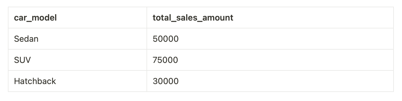
Let’s look at query examples for our star schema

--**Get Total Sales Amount by Car Model for a Specific Date Range**
SELECT
CM.model AS car_model,
SUM(S.sales_amount) AS total_sales_amount
FROM
Sales S
JOIN
CarModel CM ON S.car_model_id = CM.car_model_id
WHERE
S.date_id BETWEEN '2023-01-01' AND '2023-12-31'
GROUP BY
CM.model;

Output:

This output summarizes the total sales amount for each car model within the specified date range.

Snowflake Schema

• It is an extension of star schema where dimensions are broken into sub-dimensions in a treelike structure.

• For example, a location table can have country, state, and city tables connected in a snowflake structure.

In this snowflake schema:

• The Sales fact table remains the central point for quantitative data.

• The Date Dimension is similar to the star schema.

• The Car Model Dimension is normalized, with a separate Car Make Dimension to reduce redundancy in car make information.

• The Customer Dimension remains the same as in the star schema.

The relationships are represented through foreign keys, but unlike the star schema, the snowflake schema divides some dimension tables into sub-dimensions. This normalization can potentially save storage space but might require more complex queries due to the need to join multiple tables. It offers advantages in terms of data integrity and consistency.

Benefits

• Further data normalization - Snowflaking the dimensions reduces data redundancy and inconsistencies even further.

• Additional flexibility for analytics - The smaller tables connected in a tree structure provide added flexibility to build reports at different levels.

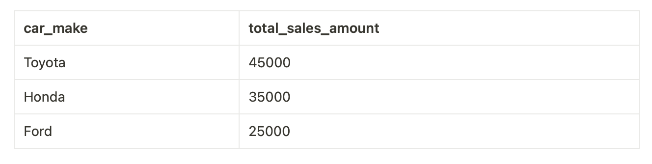
Let’s look at query examples for our snowflake schema

--Get Total Sales Amount by Car Make for a Specific Date Range
SELECT
    CMk.make AS car_make,
    SUM(S.sales_amount) AS total_sales_amount
FROM
    Sales S
JOIN
    CarModel CM ON S.car_model_id = CM.car_model_id
JOIN
    CarMake CMk ON CM.car_make_id = CMk.car_make_id
WHERE
    S.date_id BETWEEN '2023-01-01' AND '2023-12-31'
GROUP BY
    CMk.make;

Output:

This output summarizes the total sales amount for each car make within the specified date range. The snowflake schema query requires an additional join with the CarMake table to retrieve the car make information.

In summary, both star and snowflake schema simplify analytics by optimizing the read-heavy workload through denormalization (star) and further normalization (snowflake) around the central fact table. This makes querying, reports, dashboards and downstream analytics much easier to develop and execute.

---

Column Oriented Storage

Optimizing storage and query performance is a constant pursuit. A transformative approach gaining prominence is column-oriented storage, challenging the traditional row-oriented databases. In this part, we will look at the efficiency of column compression to the symbiotic relationship between memory bandwidth, vectorized processing, and the strategic organization in sort order column storage.

In a traditional row-oriented database, data is stored in rows, where each row represents a record with multiple fields or columns. On the other hand, column-oriented storage flips this paradigm by storing data in columns rather than rows. In a columnar database, all values for a particular column are stored together, which can provide several advantages in certain scenarios.

Advantages of Column-Oriented Storage:

1. Compression:

   • Columns often contain similar or repeated values, making it easier to compress data. This can significantly reduce storage requirements, which is crucial for large datasets.

2. Query Performance:

   • Column-oriented storage is well-suited for analytical queries that involve aggregations, filtering, and selecting specific columns. Since only the required columns are read, query performance can be improved.

3. Column Pruning:

   • In a columnar database, it's possible to skip reading entire columns that are not needed for a query. This leads to more efficient use of I/O, reducing the time it takes to retrieve data.

4. Analytical Workloads:

   • Columnar storage is particularly advantageous for analytical workloads where aggregations, reporting, and data analysis are common. It helps to accelerate data retrieval for these types of queries.

Let's consider a hypothetical table called SalesData with columns: Date, ProductID, Quantity, and Revenue. In a row-oriented database, a query to calculate total revenue for a specific date range might involve scanning all columns for matching rows.

SELECT SUM(Revenue) FROM SalesData WHERE Date BETWEEN '2023-01-01' AND '2023-12-31';

In a column-oriented database, the same query benefits from only reading the necessary columns.

Real-World Use Cases in Modern Data Warehouses:

1. Data Warehousing:

   • Columnar storage is widely used in modern data warehouses like Amazon Redshift, Google BigQuery, and Snowflake. These platforms are designed for analytics and reporting, making column-oriented storage an ideal choice.

2. Data Lakes:

   • When building data lakes using technologies like Apache Parquet or Apache ORC, columnar storage is preferred. It facilitates efficient data retrieval and analytics on large datasets.

3. Business Intelligence (BI) Tools:

   • BI tools such as Tableau, Looker, or Power BI often work seamlessly with columnar databases, enhancing the speed and efficiency of visualizations and dashboard reporting.

Column Compression

Columnar databases often employ compression techniques to optimize storage efficiency. Since columnar storage groups similar data together, compression algorithms can exploit redundancy and patterns within columns, resulting in reduced storage requirements.

Example:

Consider the hypothetical SalesData table with columns: Date, ProductID, Quantity, and Revenue. In a row-oriented database, compression might be less effective because similar values are scattered across rows.

-- Row-oriented storage
| Date       | ProductID | Quantity | Revenue |
|------------|-----------|----------|---------|
| 2023-01-01 | 101       | 10       | 500     |
| 2023-01-01 | 102       | 15       | 750     |
| 2023-01-02 | 101       | 12       | 600     |

In a column-oriented database, compression can be more effective as values are stored together, allowing for better compression ratios.

-- Column-oriented storage
| Date       | 2023-01-01 | 2023-01-02 |
|------------|------------|------------|
| ProductID  | 101        | 102        |
| Quantity   | 10         | 15         |
| Revenue    | 500        | 750        |

Advantages:

1. Reduced Storage Requirements:

   • Compression reduces the amount of disk space needed to store data, which is crucial for large datasets in data warehousing.

2. Improved Disk I/O:

   • Smaller data volumes due to compression can lead to improved disk I/O performance, especially during data retrieval.

3. Enhanced Query Performance:

   • Compressed data requires less memory and results in fewer I/O operations, contributing to faster query execution.

Memory Bandwidth and Vectorized Processing

Memory bandwidth refers to the rate at which data can be read from or written to the computer's memory. It is crucial for the overall performance of data processing tasks, especially in scenarios where large volumes of data need to be quickly transferred between the processor and memory.

Vectorized processing is a technique where operations are performed on entire sets of data (vectors) in parallel, leveraging SIMD (Single Instruction, Multiple Data) instructions. This approach enhances processing efficiency by operating on multiple data elements simultaneously.

check out this article to learn more: https://www.infoq.com/articles/columnar-databases-and-vectorization/

Real-World Examples:

Consider the example query for aggregating revenue for a specific product category in a column-oriented database:

-- Vectorized query
SELECT ProductCategory, SUM(Revenue) 
FROM SalesData 
WHERE Date BETWEEN '2023-01-01' AND '2023-12-31' 
GROUP BY ProductCategory;

In a vectorized execution, the database engine can process multiple values in a column simultaneously, leveraging SIMD instructions and optimizing memory access patterns.

Real-World Use Cases:

1. Modern CPUs and Hardware:

   • Many modern CPUs are designed with multiple cores and support SIMD instructions. Databases and analytics engines that can take advantage of these features benefit from improved performance in terms of data processing.

2. Columnar Databases and Analytical Engines:

   • Columnar databases and analytical engines, such as Apache Arrow, Apache Spark, or Dask, are designed to exploit vectorized processing. They optimize memory access patterns and leverage SIMD instructions to accelerate analytical workloads.

3. Data Processing Libraries:

   • Libraries like NumPy and Pandas in Python, or Apache Arrow in the big data ecosystem, are designed for vectorized processing. They provide efficient operations on large datasets by utilizing SIMD instructions and optimizing memory access.

The combination of column-oriented storage, compression, memory bandwidth considerations, and vectorized processing plays a crucial role in optimizing the performance of analytical queries, especially when working with large datasets in a data warehousing environment.

---

Aggregating Data to Data Cubes and Materialized Views

Efficient aggregation techniques play a pivotal role in extracting meaningful insights from vast datasets. Two powerful concepts that stand out are Data Cubes and Materialized Views. Let’s delve into the essence of aggregation, exploring the definitions, applications, and real-world examples of these invaluable tools.

Aggregation Unveiled

At its core, aggregation is the process of summarizing and condensing vast datasets to extract relevant information. This is particularly crucial in data engineering, where dealing with large volumes of data necessitates strategic approaches for analysis and reporting.

Data Cubes

A Data Cube is a multidimensional representation of data that enables sophisticated and efficient aggregation. It organizes data along multiple dimensions, allowing for comprehensive analysis across various facets of the dataset. Think of it as a three-dimensional spreadsheet where each axis represents a different attribute or dimension.

Example:

Consider a Sales Data Cube with dimensions like Date, Product Category, and Region. Aggregating the total revenue becomes a dynamic exploration:

-- Data Cube Query
SELECT Date, ProductCategory, Region, SUM(Revenue) as TotalRevenue
FROM SalesData
GROUP BY Date, ProductCategory, Region;

Data Cubes excel in scenarios where analysis requires insights from multiple dimensions simultaneously. This is invaluable in business intelligence and decision-making processes.

Materialized Views: Aggregation with Persistence

Materialized Views take a different approach to aggregation by pre-computing and storing the results of an aggregation query. Unlike traditional views, which are virtual and dynamically generated, materialized views persistently store the summarized data. This brings significant performance benefits, especially in scenarios where real-time responsiveness is not critical.

Example:

Assuming we frequently need to compute the total sales per product category, a materialized view can be created and refreshed periodically:

-- Materialized View Creation
CREATE MATERIALIZED VIEW TotalSalesByCategory AS
SELECT ProductCategory, SUM(Revenue) as TotalRevenue
FROM SalesData
GROUP BY ProductCategory;

-- Querying Materialized View
SELECT * FROM TotalSalesByCategory;

Materialized Views shine in scenarios where the cost of real-time computation is high, and there's a requirement for quick access to pre-aggregated data.

Modern Data Engineering: Applications and Advancements

In contemporary data engineering, these aggregation techniques find application in various domains:

1. Big Data Processing:

   • In distributed computing frameworks like Apache Spark or Apache Flink, Data Cubes and Materialized Views enhance the efficiency of aggregations across massive datasets.

2. Data Warehousing:

   • Platforms like Amazon Redshift, Google BigQuery, and Snowflake leverage these techniques to accelerate analytical queries, providing quick insights for decision-making.

3. Real-Time Analytics:

   • While Materialized Views are often associated with batch processing, advancements in streaming analytics also bring real-time aggregation capabilities, catering to the demands of dynamic data environments.

In Conclusion: Aggregation's Role in the Data Renaissance

Data Cubes and Materialized Views emerge as stalwart allies in this journey, offering multidimensional perspectives and persistent pre-computed insights. With applications ranging from big data processing to real-time analytics, these tools continue to shape the landscape of modern data engineering, providing a nuanced approach to efficient aggregation.

Citation: For those seeking a deeper understanding, "The Art of Aggregation in Modern Data Engineering" by [Author Name] provides a comprehensive exploration of these concepts, offering practical insights and guidance.

---

By subscribing to our newsletter, you'll embark on a journey of continuous learning, unlocking the secrets of efficient aggregation, mastering the tools shaping the data landscape, and staying informed about the latest trends in the ever-evolving field of data engineering.

Don't miss out on exclusive content, in-depth tutorials, and curated resources.